Orthogonal Range Searching

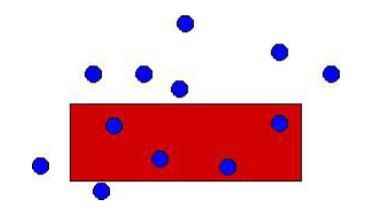
Definition A query asking to report all records whose fields lie between specified values, then transforms to a query asking for all points inside a $d$-dimensional axis-parallel box. Such a query is called a rectangular range query, or an orthogonal range query in CG.

Normalization $x$- and $y$-coordinates of points can be replaced by integers $1,2,3,\cdots, n$ in $O(n\log n)$ time (First sort and re-index). When querying, the coordinates of of the rectangle corners can be transformed to appropriate integers in $O(\log n)$ time.

In the remainder of this section we assume that no two pints in $P$ have the same $x$-coordinate, and no two points have the same $y$-coordinate.

Kd-Trees

Basic Definition

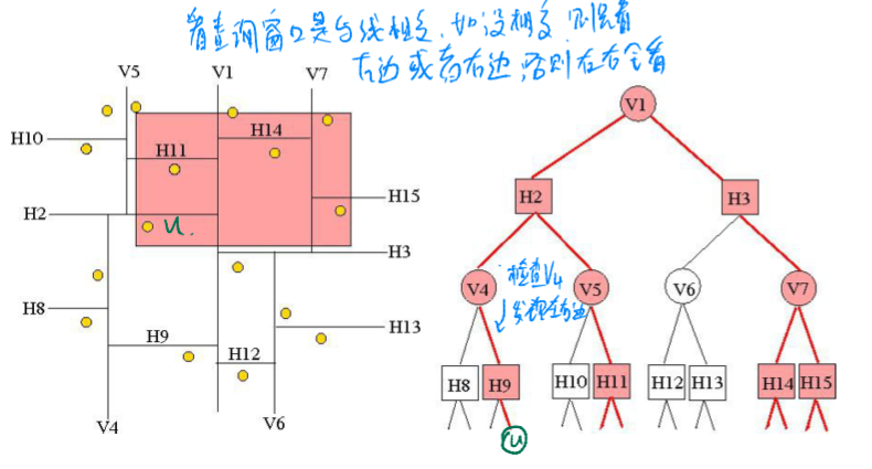
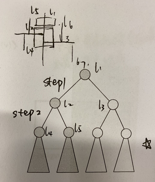
A Kd-Tree looks like:

Every vertical/horizontal line split current graph into two parts each with equal number of points on both sides until each partition contains only one point. Each node in Kd-tree represents a line. The nodes in even length from root represent the vertical line and others on odd length represent the odd line.

Preprocessing Time

The most expensive step is performed at every recursive call is finding the splitting line. This requires determining the median $x$-coordinate or the median $y$-coordinate, depending on whether the depth is even or odd. We find the median in linear time relative simply in such way, sort by $x$- and $y$- coordinates independently. Hence, the building time $T(n)$ satisfies the recurrence:

$$ T_n=\begin{cases} O(1), & if\quad n=1\\ O(n)+2T(\lceil n/2\rceil), & if \quad n>1 \end{cases} $$

which solves to $O(n\log n)$. Here $O(n)$ is the expense for median finding and recursive expression $T(\lceil n/2\rceil)$ shows the left and right build procedure.

Space: Binary tree with $n$ leaves. $O(n)$ space.

Lemma A Kd-tree for a set of $n$ points uses $O(n)$ storage and can be constructed in $O(n\log n)$ time.

Query Time

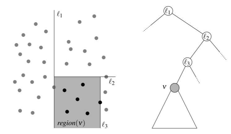
The region of a node $v$, denoted as $region(v)$, in Kd-Tree is:

Such a $region(v)$ is formed by the line represented by the ancestor nodes of $v$.

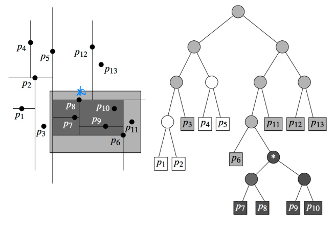
The query algorithm is: we traverse the Kd-Tree, but visit only nodes whose region is intersected by the query rectangle. When a region is fully contained in the query rectangle, we can report all the points stored in its subtree. When the traversal reaches a leaf, we have to check whether the points stored at the leaf is contained in the query region and, if so, report it.

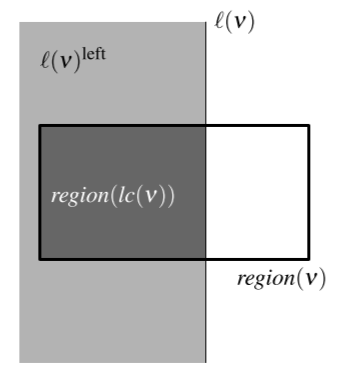
The main test of the query algorithm performs is whether the query range $R$ intersects the region corresponding to some node $v$. One can maintain the current region through the recursive calls using the lines stored in the internal nodes. For instance, the region corresponding to the left child of a node $ν$ at even depth can be computed from $region(ν)$ as follows:

$$ \operatorname{region}(l c(v))=\operatorname{region}(v) \cap \ell(v)^{\text {left }} $$

where $\ell(v)$ is the splitting line stored at $v$, and $\ell(v)^{left}$ is the half-plane to the left of and including $\ell(v)$.

The time we need to traverse a subtree and report the points stored in its leaves is linear in the number of reported points, which is $O(k)$. Besides, it remains to bound the number of nodes visited by the query algorithm that are not in one of the traversed subtrees. To analyze the number of such nodes, we shall bound the number of regions intersected by any vertical line.

Let $\ell$ be a vertical line, and let $\mathcal{T}$ be a Kd-Tree. Let $\ell(root(\mathcal{T}))$ be the splitting line stored at the root of the Kd-Tree. Observe that if the line $\ell$ intersects, for instance $region(lc(root(\mathcal{T})))$, then it will always intersect the regions corresponding to both children of $lc(root(\mathcal{T}))$, e.g., the region between line $\ell_1, \ell_4$ and $\ell_1,\ell_5$.

Define $Q(n)$ as the number of intersected regions in a Kd-Tree storing $n$ points whose root contains a vertical splitting line. To write recurrence for $Q(n)$ we have to go down two steps in the tree. Each of the four nodes at depth two in the tree corresponds to a region containing $n/4$ points.

Two of the four nodes correspond to intersected regions (at least two regions would be intersected by such region that we mentioned earlier), so we have to count the number of intersected regions of the remaining 2 nodes ($Q(n/4)+Q(n/4)$) in these subtrees recursively (the region to the left of $\ell_4$ and $\ell_5$). Hence, $Q(n)$ satisfies the recurrence

$$ Q(n)=\begin{cases} O(1), &if \quad n=1\\ 2 + 2Q(n/4), &if \quad n>1 \end{cases} $$

This recurrence solves to $Q(n)=O(\sqrt{n})$. In other words, any vertical line intersects $O(\sqrt{n})$ regions in a Kd-Tree.

Theorem A Kd-Tree for a set $P$ of $n$ points in the plane use $O(n)$ storage and can be built in $O(n\log n)$ time. A rectangular range query on the Kd-Tree takes $O(\sqrt n+k)$ time, where $k$ is the number of reported points. If its $d$-dimensional, the query time is bounded by $O(n^{1-1/d}+k)$.

1-Dimensional Range Search

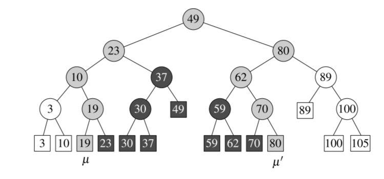
Above data structure is a BST and we call it Threaded Binary Tree .

For a 1-dimensional range query, $[u,u’]$, we first binary search $u$ in the tree, for each node $v$, report nodes in $rc(v)$ . Then search $u’$ and report all nodes in $lc(v)$.

Theorem Let $P$ be a set of $n$ points in 1-dimensional space. The set $P$ can be stored in a balanced BST, which uses $O(n)$ storage and has $O(n\log n)$ construction time, such that the points in a query range can be reported in time $O(k+\log n)$, where $k$ is the number of reported points.

Range Tree

The range tree is:

The main tree $\mathcal{T}$ is a balanced binary search tree built on the $x$-coordinate of the points in $P$.
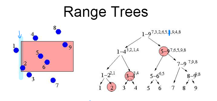
For any internal or leaf node $v\in \mathcal{T}$, the canonical subset $P(v)$, which is the subset of points store in the leaves of the subtree rooted at a node $v$, is stored in a balanced associated BST $\mathcal{T}(v)$ on the $y$-coordinate of the points. The node $v$ stores a pointer to the root of $\mathcal{T}(v)$, which is called the associated structure of $v$.

Space Because 1-dimensional range trees use linear storage it follows that the associated structures of all nodes at any depth of $\mathcal{T}$ together use $O(n)$ storage. The depth of $\mathcal{T}$ is $O(\log n)$. Hence, the total amount of storage required is bounded by $O(n\log n)$.

Preconstruct Constructing a BST from an unordered list is $O(n\log n)$ but if the list is sorted, it could be reduced to $O(n)$. Thus, for this two level structure, we first sort the $x$-coordinate and $y$-coordinate and then we build the first level-tree and second level tree in $O(n)$, totally $O(n\log n)$.

Query First selects $O(\log n)$ canonical subsets that together contain the points whose $x$-coordinate lie in the range $[x,x’]$, This can be done with the 1-dimensional query algorithm. Of those subsets, we then report the points whose $y$-coordinate lie in the range $[y,y’]$ using same methods. Thus in total $O(\log^2n+k)$.

Theorem Let $P$ be a set of $n$ points in the $d$-dimension. A range tree for $P$ uses $O(n(\log n)^{d-1})$ storage and can be constructed in $O(n(\log n)^{d-1})$ time. By querying this range tree one can report the points in $P$ that lie in a rectangular query range in $O(\log^dn+k)$ time, where $k$ is the number of reported points.

Improved Range Tree

Fractional Cascading

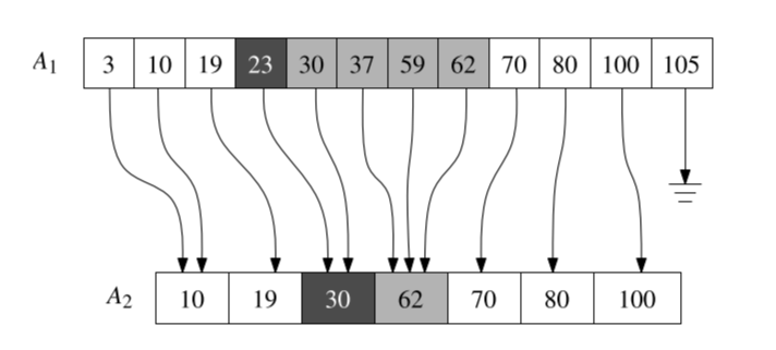
Let $S_1$ and $S_2$ be two sorted lists of numbers. Generally, if we want to report all objects in $S_1$ and $S_2$ whose keys lie in a query interval $[y,y’]$, we need to do two binary searches with $y$ in $S$ and and walk along $S$ until $y’$. The total time is $O(k)$ plus the time for two binary searches, one in $S_1$ and the other in $S_2$.

If, however, the keys of the objects in $S_2$ are a subset of the keys of the objects in $S_1$, then we can avoid the second binary search as follows. We add pointers from the entries in $S_1$ to the entries in $S_2$: if $S_1[i]$ stores an object with key $y_i$, then we store a pointer to the entry in $S_2$ with the smallest key larger than or equal to $y_i$. If there is no such key, then the pointer from $S_1[i]$ is $nil$. Then in the search of $S_2$, we just follow the pointer created in process of $S_1$, which takes only $O(1+k)$ time.

Range Tree has exactly such structure. We use Fractional Cascading to improve it.

After sorted in preprocessing, The second-level structure is always the subset of its ancestor nodes. Since we find the same nodes, in the first level binary search we can position the node we should start search in second level. For example, in root node, we find 2 as the left most point, and the pointer in 2 points to 6 since we have sorted it in $y$-monotone already.

Theorem Let $P$ be a set of $n$ points in $d$-dimensional space, with $d\geq 2$. A layered range tree for $P$ uses $O(n\log^{d-1}n)$ storage and it can be constructed in $O(n\log^{d-1}n)$ time. With this range tree one can report the points in $P$ lie in a rectangular query range in $O(\log^{d-1}n+k)$ time, where $k$ is the number of reported points.

Reference:

Orthogonal Range Search, CG - Lecture, UCPH-DIKU.
Chan’s paper

Thomas Men

$\int_{birth}^{death}\text{study} dt = \text{life}$